RecordBuffer - A Data Serialization Approach in DataMine

03 Jan 2016

Data serialization is a basic problem that every data system has to deal with. To provide an efficient solution, a data serialization approach should be able to arrange the data into a compact binary format which is independent of any particular application. Nowadays there are some open-source projects on the data serialization system, such as Avro, Protocol Buffer and Thrift. These projects have reasonable large communities and are rather successful in different application scenarios. They are generally applicable in different applications, more or less following the similar ideas when serializing the data and providing APIs for message exchanges. These approaches are for general purpose and usually working well. Additionally it is also possible for them to work with other data formats such as Parquet to provide variety of options.

However, they could do better when applied to the data with nested structure. For example, the in-memory record representation may consume the similar memory even though only a few of columns have meaningful values. On the other hand, it is possible to improve the deserialization performance with the help of index.

DataMine, the data warehouse of Turn, exploits a flexible, efficient and automated mechanism to manage the data storage and access. It describes the data structure in DataMine IDL, follows a code generation approach to define the APIs for data access and schema reading. A data encoding scheme, RecordBuffer is applied to the data serialization/de-serialization. RecordBuffer depicts the content of a table record as a byte array. Particularly RecordBuffer has the following structure.

• Version No. specifies what version of schema this record uses; it is required and takes 2 bytes.
• The number of attributes in the table schema is required and takes 2 bytes.
• Reference section length is the number of bytes used for the reference section; it is required and takes 2 bytes.
• Sort-key reference stores the offset of the sort key column if exists; it is optional and takes 4 bytes if exists.
• The number of collection-type attributes uses 1 byte for the number of collections in the table, and it is required.
• Collection-type field references store the offsets of the collections in the table sequentially; note that the offset of an empty collection is -1.
• The number of non-collection-type field reference uses 1 byte for the number of non-collection-type columns which have hasRef annotation.
• Non-collection-type field references sequentially store the ID and offset pair of columns with hasRef annotation if exist.
• Bit mask of attributes is a series of bytes to indicate the availability of any attributes in the table.
• Attribute values store the values of available attributes in sequence; note that the sequence should be the same as that defined in the schema.

Different from other encoding schemes, RecordBuffer has a reference section which allows index or any record-specific information. Having index in the reference section can locate the field (like sort-key) directly, simplifying data de-serialization significantly. On the other hand, the frequently-accessed derived values can be stored in the reference section to speed up data analytics. This is quite useful when nested data are allowed. For example, a summary on the nested attribute values can be derived and stored in the reference section, such that the deserialization of the nested table (usually very costly) can be avoid when applying aggregation to the attribute.

Deploy Application As Data (DaaD)

11 Nov 2015

The distributed computing stack commonly uses a layered structure. A functionally independent component is defined on each layer, and different layers are connected through APIs. This structure makes it quite easy for system to scale. One example of such a system can be composed of local OS/FS, distributed FS, resource management system, distributed computing frameworks, and applications. Nowadays, the HDFS is often used as the distributed file system. Yarn is one example of the resource management systems, whereas Spark can be one of promising computing frameworks.

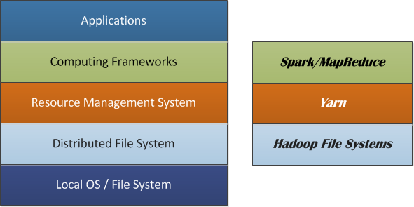
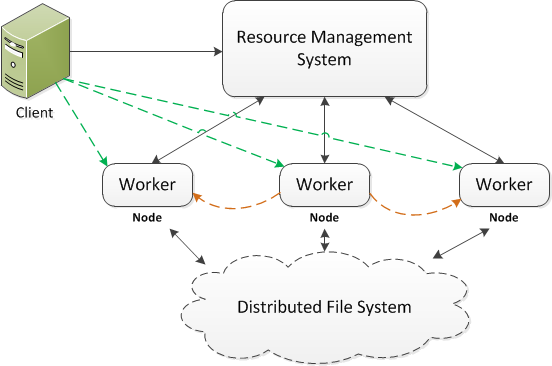
The key of distributed computing is to run the same code on the different parts of data then aggregate the results into the final solution. Particularly, the data are first partitioned, replicated and distributed across the cluster nodes. When an application is submitted, the resource management system decides how much resource is allocated and where the code can be run (usually on the nodes where the input data are stored, so called data locality). The computing framework devises a job or work plan for the application, which may be made up of tasks. More often than not a driver is issued in the client side (e.g., lines in green) or by a worker (e.g., lines in orange). The driver initializes the job and coordinates the job and task execution. Each task is executed by a worker running on the node and the result can be shuffled, sorted and copied to another node where the further execution would be done.

There are two popular ways to deploy the application code for execution.

1. Deploy the code in the cluster nodes - This approach distributes the application to every node of the cluster and the client server. In other words, all involved nodes in the system have a copy of the application code. It is not common, but in some cases it is necessary when the application depends on the code running in the node. The disadvantages of this approach are obvious. First the application and the computing system have a strong coupling, such that any change from either side could potentially cause issues to the other. Second, the code deployment becomes very tedious and error prone. Think about the case where some nodes in the distributed environment fail during the code deployment. The state of cluster becomes unpredictable when those failed nodes come alive with the old version of code.
2. Deploy the code in the client only - A more common strategy is to deploy the application code to client server only. When running the application, the code is first distributed to the cluster nodes with some caching mechanism, such as the distributed cache in the Hadoop. This simple but effective approach could decouple the application and its underneath computing framework very well. However when the number of clients is large, the deployment can become nontrivial. Also if the size of application is very large, the job may have a long initialization process as the code needs distributing across the cluster.

DaaD: Deploy Application As Data

In the distributed computing, the code and the data are traditionally treated differently. The data can be uploaded to the cloud and then copied and distributed by means of the file system utilities. However the code deployment is usually more complex. For example the network topology of application nodes must be well defined beforehand. A sophisticated sync-up process is often required to ensure the consistency and efficiency, especially when the number of application nodes is large.

Therefore if the code can be deployed as data (i.e., DaaD), the code deployment can be much simpler. The DaaD is a two-phase process.

1. The application code is uploaded to the distributed file system just as common data files.
2. When running the application, a launcher is used to load the code from the distributed file system, store the code in the distributed cache accessible to all nodes and issue the execution on node.

Clearly, the launcher is required to deployed to the client where the execution request is submitted. It should be independent of any specific applications. An example can be found at DaaD¹.

The improvement by the DaaD can be significant.

• The deployment becomes much simpler. Often the code can be uploaded to the distributed file system through a simple command. Then the code replicating and distributing can be achieved automatically through the file system utilities.

• The launcher can be defined as a simple class or executable file, which is quite stable. It is trivial to distribute it to the application node.

• The application code is loaded for execution only if an execution request is issued. Namely the code is actually copied and distributed in the lazy way. Importantly the latest version of code is always used.

• Having no local copy can avoid of code inconsistency problem.

• It makes it much easier for different code versions coexist in production. Image the scenario where it is necessary to run the same application with different code versions for A-B test.

Highly Efficient User Profile Management in Petabyte-Scale Hadoop-based Data Warehouse

10 Oct 2015

Traditionally the user profile data are stored and managed in the data warehouse. The user profile can be frequently updated to reflect the changes of user attribute and behavior. Moreover, it is critical to support a fast query processing for profile analytics. These basic requirements become challenging in the big data system, as the scale of profiles have reached a point (over petabytes) that the traditional data warehousing technology can barely handle.

The challenges mainly come from two aspects: the updating process is costly as the daily change can be huge and on the other hand the query performance must keep being improved as the input is rapidly increasing. For example the daily changes in the big data system can be more than terabytes, which makes data updating very expensive and often slow (big latency).

The traditional data warehouse provides a standard solution to the problem of user profile management and analytics, however the data scale that it normally deals with is not satisfactory. The data size in the traditional data warehouse is usually up to tens of terabytes. In the big data system, the petabyte-scale data store is quite normal, such that it is difficult for the traditional data warehouse to store and manage so many user profiles in an efficient way.

At Turn, we come up with an integrated solution to the highly efficient user profile management. Basically we build a data warehouse based on the Hadoop file systems. The size of data stored in the data warehouse can be on a petabyte scale. The data can be stored in row-based or columnar layouts in the data warehouse, such that it can provide both an efficient updating performance and a fast profile analytics.

Architecture

The architecture of the profile management system is mainly composed of the following components:

1. Operational Data Store (ODS)
2. Analytics Data Store (ADS)
3. Parallel ETL
4. Cluster Monitor
5. Database
6. Query Dispatcher
7. Analytics Engine

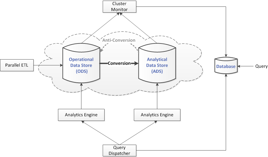
Every day there is a huge amount of data generated from the front-end system, like ad servers. The Parallel ETL (PETL) is a process running in the cluster to collect and process these data in parallel and store them in the Operational Data Store (ODS). The status of the PETL, like what data have been processed, is collected by the cluster monitor and kept in the Database.

The ODS is a row-based storage, as it must support a fast ingestion of the incoming updates. The key-value store can be faster in the data updating, however it is much slower for data analytics. In the case of profile management, the update can be merged into the profile store (i.e. ODS) regularly in batch mode. The cluster monitor collects the status of the ODS, like what data have been stored, what queries have been executed etc, and stores them in the Database.

The Analytical Data Store (ADS) provides a better solution to the data analytics. In the ADS, data are stored in columns. Comparing with its row-based counterpart (i.e., the ODS), the columnar store has a better compression ratio when storing the data, therefore has smaller data size. More importantly, only the data of interested are loaded and read when executing the user query on the columnar store. The disk I/O cost saving is almost optimal, therefore in the I/O intensive application it can achieve faster execution time in orders of magnitude comparing with the ODS. The cluster monitor collects the status of the ADS, like what data have been stored, what queries have been executed etc, and stores them in the Database.

As the data have different layouts in the ODS and the ADS, there is a data conversion from the ODS to the ADS. The conversion result is merged with the data in the ADS. Note that the ADS may not have the latest update in the ODS because the data conversion is done in batch mode. The cluster monitor collects the status of the conversion job and stores it in the Database.

When a user query is submitted, it is first stored in the query table of the Database. The query dispatcher keeps scanning the Database to (1) decide which query to execute next based on the factors, such as the waiting time, the query priority, etc, (2) decide which data store (i.e., ODS or ADS) to use for the query execution based on the data availability and the cluster resource availability, and (3) send the query job to the analytics engine for query execution.

Both the ODS and the ADS have an analytics engine to execute the query job from the query dispatcher.

The Database stores all the status information, including (1) the submitted query job, (2) the status of cluster, (3) the status of data stores (the ADS and the ODS), (4) the status of jobs running in the cluster, including the PETL, the converter, etc.

Disaster Recovery across Data Centers

04 Jun 2015

In the era of BigData, the data storage becomes so large that recovery from a disaster, such as the power outage of a data center, becomes very difficult. The traditional transaction-oriented data management system relies on a write-ahead commit log to record the system state and the recovery process will work only if the log processing is faster than the incoming change requests. In other words, commit log based approach hardly works for big data system where terabytes of non-transactional daily changes are norms.

In Turn, we exploit a geographically apart master-slave architecture to support high availability (HA) and disaster recovery (DR) in the large scale Hadoop-based DWS (Data Warehouse System).

The master and the slave are located in the different data centers that are geographically apart. Functionally, the slave is like a mirror of the master. The master or slave is composed of a Hadoop cluster, a relational database, an analytics engine, a cluster monitor, a query dispatcher, a parallel ETL component, and a console. Not all of these components in the slave are active. For instance, the cluster monitor in the slave is standing by, whereas its analytics engine should be active to accept query jobs.

Data replication happens from the master to the slave to assure the data consistency between the Hadoop clusters, and database replication reflects any change on the master database to the slave database. The master and slave are connected with a dedicated high-speed WAN (Wide Area Network).

The master-slave architecture makes DR and HA possible when one of the data centers fails. Additionally the workload balancing between master and slave optimizes the query throughput¹.

Failover and Disaster Recovery

Failure is common in the large storage system. It could be due to hardware failure, software bug, human error etc. The master-slave architecture makes the HA and DR possible and simple in the petabyte-scale data warehouse system at Turn.

Network Failure

When the WAN fails completely, a performance degrading can occur as all queries will be dispatched to the master only. The data and database replications also stop. Fortunately nothing special has to be done with the Hadoop cluster when the WAN comes back to normal, because the data replication process will catch up with the missing data of the slave. A sync-up operation is triggered to synchronize the slave database with the master database.

Hadoop Cluster Failure

In case of the Hadoop cluster failure in the slave, the DWS keeps working as the master has everything untouched. It is a little complex when the master loses its Hadoop cluster, as it implicates a master-slave swapping. Particularly, all components of the slave become active and take over the interrupted processes. For instance, parallel ETL becomes active first, starting to ingest data. Importantly during the swapping, the DWS keeps accepting and running the user query submission.

When the failed Hadoop cluster comes back, the data replication process can help to identify and copy the difference from the current master to the slave. Depending upon the downtime and data loss caused by the failure, it can take up to days to complete the entire recovery. However, certain queries can be executed in the recovering cluster. Furthermore based on the query history in the relational database, the hot-spots of data can be recovered first.

Data Center Failure

It is rare but fatal if one of the data centers fails. At Turn the DWS tolerates a failure of either the master or the slave. When the slave data center is down, the performance is degraded because only one of the Hadoop clusters is available and all workload are moved to the working one. The data recovery is trivial because the replication processes will catch up the difference once the failure is fixed.

If the master data center fails, the stand-by services in the slave will become active right away. There is a chance that data or query may lose if the failure happens in the middle of the data replication. However, the loss can be mitigated if the replication is scheduled to run more frequently. After all services are active, the slave becomes the master. When the failed data center is recovered, it will run as a slave. The data replication is issued to transfer the difference over. Before the database replication starts, a database sync-up process is required to make the new slave have the same content in its relational database.

Efficient Distributed Copy across Data Centers

20 May 2015

DistCp is a tool used for large inter/intra-cluster data transfer. It uses Map-Reduce to effect its distribution, error handling and recovery, and reporting. ¹

Currently DistCp is mainly used for transferring data across different HDFSs (HaDoop File Systems). The HDFSs can sit in the same data center where the data flow through LAN (Local Area Network) or in the different data centers connected by WAN (Wide Area Network). Basically, DistCp issues Remote Procedure Calls (RPCs) to the name nodes of both source and destination, to fetch and compare file statuses, to make a list of files to copy. The PRC is often very expensive if the name nodes are located in the different data centers, for example, it could be up to 200x slower than the case within the same date center in our experience. DistCp may issue the same RPCs more than once, dragging down the entire performance even further. DistCp doesn’t support regular expression as input. If the user wants to filter and copy files from different folders, she has to either calculate a list of file paths beforehand or execute multiple DistCp jobs. Moreover DistCp allows preserving the file attributes during the data transfer. However, it does not preserve time stamp of file, which is quite important in some applications.

To address these problems with DistCp, we introduced an enhanced version of distributed copy tool, DistCp+². Particularly DistCp+ makes it easier and faster to transfer a large amount of data across data centers. Comparing with DistCp, DistCp+ introduces improvement in the following aspects:

Support Regular Expression

A regular expression is a sequence of characters that forms a search pattern. It has been wildly used in the text processing utilities, for example the command grep in Unix. The regular expression used by DistCp+ is based on the syntax of regular expression in Java ³ with minor changes. To use the regular expression option with DistCp+ you must specify 2 parameters: a root URI and a path filter. The path filter follows normal regular expression rules but treats all ‘/’ tokens in a special way. The ‘/’ token is used as a delimiter and the regular expression provided is split into multiple sub-expressions around this token. Each sub-expression is used as a separate path filter for a specific depth relative to the URI with the leftmost sub-expression being used first.

For example, assuming you specify “/logs/” as the root URI and provide a regular expression of “server1|server2/today|yesterday”. The regular expression will be split into the 2 sub-expressions “server1|server2” and “today|yesterday”. Then DistCp+ will traverse the file system starting at the root (“/logs/”) and use any file that matches the first sub-expression (“server1|server2”). Folders are recursively expanded, but at each new depth in the file system the next sub-expression is used as the path filter. Using this example provided, you can match such files as “/logs/server1/yesterday” and “/logs/server2/today”, but it will not match something like “/logs/yesterday”. Also note that if a folder matches the last path filter, the entire folder is used as input instead of being recursively traversed.

Cache File Status

When a DistCp job copies a large number of files especially across geographically distant data centers, it usually has a very long setup time as several RPCs are issued to collect the file status from both sides. However, the cost of RPC is very high especially when it is through WAN. DistCp repetitively issues RPCs to get individual directory or file’s status object. These RPCs either overlap with previous ones or can be combined into fewer RPCs. To reduce the cost, a cache of file status is created in the early stage, when directory level RPC is used to get all file status under the very directory in one RPC. Then RPC is necessary only if a cache miss occurs in the following stages. For tens of thousands file transferring, we observe a significant improvement on the end-to-end time cost.

Keep Time Stamp

DistCp supports to preserve the file status, including block size, replication factor, user, group and permission. However, it does not keep the time stamp (or last modified time stamp) of the file, which is important especially when we use “-update” option to skip files without any change. Checking CRC (Cyclic Redundancy Check) of the file is an alternative, but the CRC computation of files is too high to be practical for large data transfer. Comparing the file size may not be accurate as some changes do not change the size of files. Therefore the time stamp is better to decide if an update is necessary. Particularly, the file has its time stamp preserved after copied if necessary. When “-update” option is specified, DistCp+ compares the time stamps of files on different clusters to decide if the file is included.

In Turn, DistCp+ has been used to transfer data among different data centers regularly. A DistCp+ job can usually copy thousands of files from different folders and the data volume can be terabytes.